HAPMIXMAP

a program to model HapMap haplotypes using tag SNP genotype data

Using HAPMIXMAP to test all loci in a candidate gene in which tag SNPs have been typed in cases and controls

Data files

The dataset consists of a case-control study in which 1000 individuals of European ancestry were typed at 9 SNPs in a candidate gene on chromosome 7. These 9 SNPs were chosen as tag SNPs, using the program TAGGER, based on an early version of the HapMap. There are four files in the 'data' directory:

dn_loci.txt - a locusfile containing loci around the region typed.
dn_genotypes.txt - a genotypesfile containing CEU (European) HapMap genotypes for the loci in the locusfile.
CaseControlGenotypes - a ccgenotypesfile with genotypes for the case-control individuals.
outcome.txt - a binary outcomevarfile containing case/control indicators for the typed individuals.

These files are already prepared for analysis by HAPMIXMAP. To produce them, the following steps are required. See here for details on file formats.

Download the HapMap haploid data file for the chromosome containing the SNPs and the continental group that was sampled in the case-control study
Extract all hapmap data for the region containing the typed SNPs, including 100 kb on either side of the sequence of typed loci, and write out this file in HAPMIXMAP format. For this example, we obtain a file of 298 loci spanning 160 kb.
Write a table of these loci in HAPMIXMAP format.
Drop any loci from the raw genotypes file that are not matched in the HapMap. Recode the alleles in the raw genotypes file so that the numeric coding corresponds to that in the HapMap database, sort by map position, and write file genotypes.txt in HAPMIXMAP format
Write a file containing values of the outcome variable.

All these steps, except the last, can be automated using the conversion tools supplied as follows:

Data Preparation

This is only a brief guide; more detailed instructions are given in the hapmixmapFormatter/README.txt file. Also supplied in the data directory is rawgenotypes.txt, which is the same as CaseControlGenotypes.txt but with genotypes coded as bases (e.g. A:G instead of "1,2"). It is necessary to supply them like this to ensure consistency of encoding with the HapMap genotypes. You will need an internet connection for the download step to work and you will need gzip available to unzip the downloaded files. The typed loci are on chromosome 7 so we need '-c=7' and the individuals are Europeans so we need the population code -p=CEU. We are downloading, unxipping and formatting so wee need the '-d', '-u' and '-f' flags. We will gve the output files different names so they don't overwrite the originals. You should find they are identical.

perl hapmixmapFormatter/getdata.pl -c=7 -p=CEU -d -f -u -genotypesfile=data/copyGenotypes.txt -locusfile=data/copyLoci.txt -gdata/rawgenotypes.txt -ccgfile=data/copyCCGenotypes.txt

A full list of options for the script can be produced by typing:

perl hapmixmapFormatter/getdata.pl -h

You can also invoke the conversion program FPHD directly once you have downloaded and unpacked the HapMap data. A full list of options for this program can be produced by typing:

hapmixmapFormatter/FPHD -h

Running the analysis

To reduce the time taken for the program to converge, we undertake an initial run using only the phased HAPMAP haplotypes and save a single draw from the posterior distribution of model parameters. The saved values are used as initial values for the subsequent run in which the posterior distribution is generated given both HAPMAP haplotypes and diploid case-control genotypes at tag SNPs. The instructions below assume that the hapmixmap executable and the R script, AdmixmapOutput.R, are in the same directory you are working in (as they will be if you have just unpacked the binary package or built from the source package).

For the first run, type

./hapmixmap training-initial.conf

This short run starts the sampler and stores a final draw from the sampled distribution of model parameters for use as initial values in the next run

When this short initial run has completed, type

./hapmixmap training-resume.conf

then type

R CMD BATCH --vanilla AdmixmapOutput.R results/Rlog.txt

to run the R script that processes the output files.

Note the value of the posterior mean of the "energy" (minus the log-likelihood of the model parameters given the data), which is written to the log and to the console.

Repeat the training run by typing hapmixmap training-resume.conf
analysis until the energy is no longer falling with each new run.

then type

R CMD BATCH --vanilla AdmixmapOutput.R results/Rlog.txt

to run the R script that processes the output files.

The results of each run are written to the folder results. Results of previous runs will be overwritten unless you rename the results directory or use the option 'deleteolddata=0'.

To determine whether the program has been run with a long enough burn-in, examine the plot of the realized values of "energy" that has been written to the file EnergyTracePlot.ps. If there is a downward trend, the burn-in was too short. Another check is to look at the Geweke diagnostics for the global model parameters in the file ConvergenceDiagnostics.txt: For each parameter, the test compares the mean over the first 10% of iterations (after the burn-in) with the mean over the last 50% of iterations.

For the case-control analysis, type

./hapmixmap testing.conf

When this has completed, run the R script again

Interpretation of results of score tests

To view the output you will need a postscript viewer such as Ghostview.

To determine whether the program has been run long enough for the score tests to be computed accurately, open the file TestAllelicAssociations.ps with a postscript viewer and examine the plot of log p-values based on all iterations so far. If the program has been run long enough, the p-values will have stabilized: that is, the plot of cumulative results should be horizontal lines by the end of the run.

The file PosteriorQuantiles.txt contains the posterior means, medians and 95% credible intervals for the global model parameters. The number of arrivals per megabase (Mb) is inferred as about 60. This is equivalent to an average haplotype block length of about 19 Kb (1000 / (60 x 7/8) ).

To evaluate the extent to which our tag SNP panel has extracted information about associations with HapMap loci, we look at the file InfoExtractedMap.ps

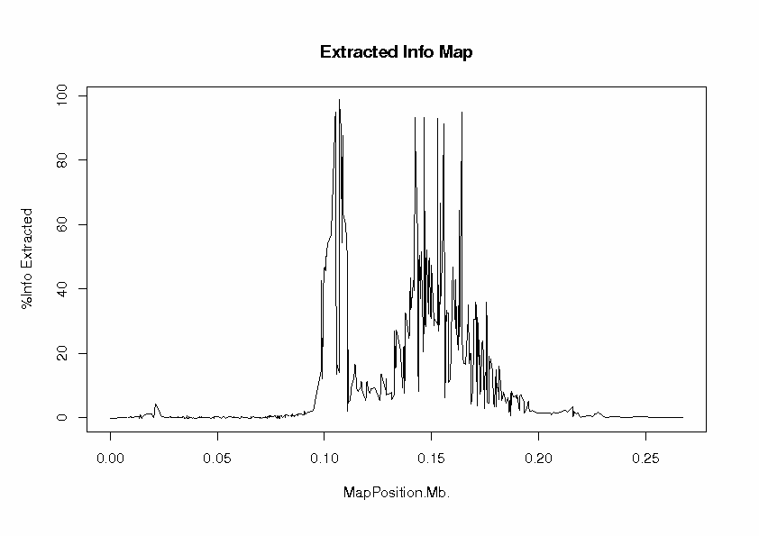
At each locus, the proportion of information extracted is the ratio of observed information to complete information in the score test. This can be interpreted as a measure of the efficiency of the study design, compared with a design in which the locus has been typed directly. The "information" here is Fisher information, defined as the expected value of minus the second derivative of the log-likelihood with respect to the parameter under test, which is the regression parameter b for the effect of allele 2 (coded as 0, 1, 2 copies). The log-likelihood function is evaluated at the null value, b = 0, of the parameter under test, which is the effect of the locus in an additive regression model). The peaks are the 9 typed loci, at which nearly 100% of information has been extraced, as one would expect. For some of the untyped loci, some useful information has been extracted, but there is a large gap in coverage of the candidate gene region between about 0.11 and 0.13 Mb. The information extracted falls off to zero beyond about 200 kb from the first and last typed loci.

Next we can examine the haplotype structure of the region, shown in the file ArrivalRateMap.ps

The spikes of high arrival rates represent boundaries between haplotype blocks (sometimes interpreted as recombination hotspots). There is a block boundary at about 0.11 Mb, and the tag SNPs do not adequately cover the region to the right of this boundary.

The results of the tests for associations are contained in the file AllelicAssociationTestsFinal.txt. This is most easily viewed using a spreadsheet program. The table has one row per locus. The column labels are explained below

Locus: the rs number in dbSNP
Score (U): This is the gradient of the log-likelihood as a function of the regression parameter b for the effect of allele 2 (coded as 0, 1, 2 copies) at the null value, b = 0. For a case-control study, the regression model is a logistic regression, with disease status as outcome variable and any specified variables as covariates.
Complete information: This can be interpreted as a measure of how much information about b you would have if the locus had been typed directly - where the complete information is small, this is because the locus is not very polymorphic
Observed information (V): In large samples, the log-likelihood function is approximately quadratic and the maximum likelihood estimate of b is therefore approximately U / V. This approximation only holds where the observed information is reasonably large.
Percent information: This can be interpreted as a measure of the efficiency of the tag SNP panel in extracting information about the effect of the locus under study
Missing 1: This is the percent of information that is missing because of uncertainty about the genotypes, given the model parameters. This can be interpreted as a measure of the inadequacy of the tag SNP panel.
Missing 2; This can be interpreted as the percent of information that is missing because of uncertainty about the model parameters, which are inferred from the panel of 120 phased HapMap gametes. .
Standard normal deviate: This is U / √V. This value will not be computed where the the observed information is small. Where there is not enough information, the asymptotic properties of the score test do not hold.
Two-sided p-value for the standard normal deviate
ArrivalRate: posterior mean for the expected number of arrivals in the interval. Large values (> 1) indicate a haplotype block boundary or "recombination hotspot".
FreqPrecision: posterior mean for the allele frequency precision parameter for the locus. Large values (> 0.1) indicate that the state-specific allele frequencies are not all close to 0 or 1: in other words that which allele is present cannot be reliably predicted from knowing which of the 8 modal haplotypes is present. One possible explanation for large values could be that the locus has a high "mutation rate".

This table shows 180 lines of this file: the flanking regions with no information extracted have been omitted.

The test statistic and p-value are not evaluated where the proportion of information extracted is less than 10% - below this information level the asymptotic properties of the score test may not hold, and computational difficulties arise in calculating the test statistic accurately.

There's some weak evidence of association in the region containing the first three typed loci, but it's clear that we need to type more SNPs to achieve adequate coverage of this candidate gene. In the next section, we look at the results with an augmented dataset that has more typed SNPs.